[tutorials & resource material arranged by topic Class Table

Statistics: Heavy on Vocabulary and Images, Little Computation


        (Click on most images to see an enlargement.)
A Year of Statistics in an Hour or Two:
    Heavy on Vocabulary, Light on Computation, No Counting Theory

    Designed as a one hour talk/intro, for someone with an 8th grade math background. This page is heavy on the pictures, but, light on the computation.

    There's no permutations, combinations, counting theory. There are links to this stuff.

    For just the vocabulary from this page, "A Year of Statistics in an Hour or Two," go to Statistics Vocabulary.

    For statistics resources go to MIDDLE GROUND, the statistics info page.


Support Stuff/Down Load Material

      Here's the spreadsheet used for this page. Here is the pdf file of this page in case you wish to take notes. Here is a link to where the video of this page is stored.


Table of Contents In Order of Presentation
A Year of Statistics in an Hour or Two:
    Heavy on Vocabulary, Light on Computation, No Counting Theory
Population, Sample, Data, Statistic
Discrete or Continuous
Take a Samples
Look at the Data
Theoretical vs Experimental & Descriptive
    vs Analytical Statistics
Probability
More Vocabulary and Topics that Are Not Included on this Page
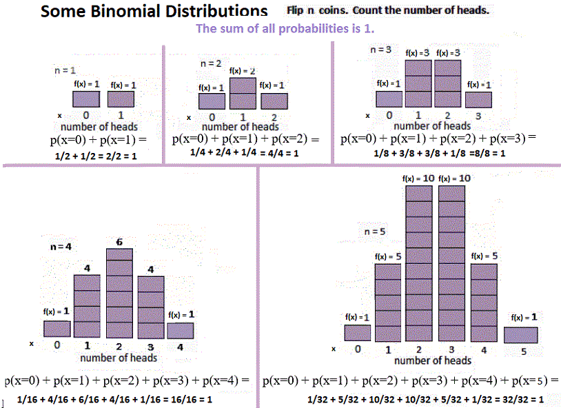
The Binomial Distribution
Thank Goodness for Probability Density Functions
Normal and Standard Normal Distributions
Confidence Intervals
Hypothesis Testing
Just the Vocabulary (Sorted Alphabetically)

 
Population, Sample, Data, Statistic

    Suppose you own a big tank of fish. You might wish to examine just one of the fish. You might examine a bunch of fish, or you might examine all the fish in a tank, the entire population. You could look at, all at one time, their color, their length, their shineyness, the number of fins on each fish, to get a big picture of the fish. This would be a look at all of the features of the fish at once and would give you a good general idea of the fish.

    If instead you looked at one feature of each fish you chose, you would be taking a STATISTICAL look at the fish. You would be considering, one at a time, DATA or something about each fish - a measurable or countable or classifiable piece of information. Data is information -- a measurements, a count, a description. You might then wish to process the collected data to compute/find a statistic about the data -- the average length, the most frequent length, the spread of lengths, the longest (or maximum) length.

    This computation could be done for either the sample (collection) of fish or for the population (all the fish). If one just took a sample or collection of fish, the sample might include by chance just one fish or all of the fish. The bunch or collection or sample of the fish would still be called a sample.

    Usually the population of stuff, like fish, or the population of raw data is too large to examine or is not avaliable and a sample or statistical sample is used to learn about the statistical population.

    If you considered the population to be the fish at the fish store, your data might be "proof" that your fish are longer, or heavier, than the fish at the store, the population, because of how you are feeding or treating your tank of fish. More on that later.


Vocabulary
  • SAMPLE - a collection - 1, more than 1, or perhaps all (here, you would know this by emptying or filling the tank).
     
  • POPULATION - a collection of all the items under consideration (here, you would know this by emptying or filling the tank).
     
  • STATISTICAL SAMPLE - a collection of raw data - counts, lengths, durations of time, test scores, integers, real numbers, etc.
     
  • STATISTICAL POPULATION - a collection of all the raw data - counts, lengths, durations of time, test scores, integers, real numbers, etc.
    One usually does not examine the entire population. Population statistics are often given in a situation. You might be studing the statistical sample.
     
  • DATA or DATA POINT or RAW DATA - 1 piece of information -- as in the length of a fish, as in the number of fins on a fish, as in the color of a fish.
     
  • STATISTIC - the processed information -- as in the average length of all the fish in the sample.


Discrete or Continuous

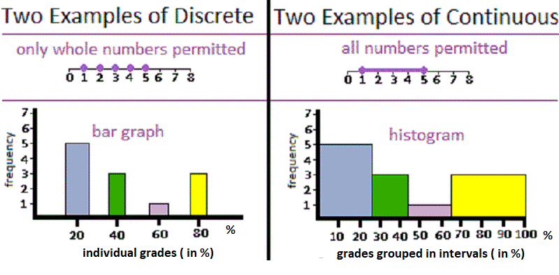
Click on the image to enlarge it.

    If you do decide to do a statistical study, two different types of data are obtained/used/needed. The type that is collected depends on what you are measuring, or counting, or observing. The two kinds of data are continuous and discrete.

    Your only task as we begin to analize data is to take note of what data is continuous and what is discrete.


Vocabulary
  • CONTINUOUS - all numbers are used over the desired interval
    You might have data that are real numbers on a range 0 < x < 6: numbers like 4.387, .58, 5.55555... or you might have real numbers from -3 to 5.
    Examples:
    ·       the length of a fish, measured in meters with a meter stick or tape
    (real numbers)
    · a length of time, as in how many months till a birthday
    · a height,
    · a weight
    · the temperatures on Wednesday mornings in January
  • DISCRETE - only certain numbers are used over the desired interval
    You might have data that are integers: numbers like -3, 0, -10, 4, 6, 10, 11, or natural (counting) numbers: numbers like 1, 2, 3, 4, ...
    Examples:
    ·       the length of fish, measured to the nearest half inch
    (whole numbers and halves only)
    ·       a number of things, as in how many nickels there are in a jar,
    (whole numbers)
    ·       a shoe size, as in 8, 8 1/2, 9, 9 1/2
    ·       a grade in school, as in: 1st, 2nd, 3rd
    ·       a night's win (+) or loss (-) in dollar bets (integers)


Take a Sample

    Here are samples of samples of fish.

    They are not however statistical samples. Statistical samples are collections of raw data -- measurements, counts, lengths of time, etc.

    Samples are used to create the data so a purely numeric picture or a graphic representations of the what's in the tank, the population, may be produced.

    Two things are important when taking a sample:

  1. Making sure the sample is large enough to ensure the accuracy you need later.
  2. Getting a random sample.

    Many things effect the size of the sample needed. On this page the sample size was chosen for educational, not statistical, purposes --to display a few important things about samples of data and what one might do with them.

    Check out the above samples of samples of fish. You might say "Two of the samples don't look very random." Those would probably be the one with the yellow fish on the bottom of the tank and the ones with only the yellow and white fish. But, these might indeed be random samples.

    When average citizens thinks of a random sample, they think of a sample with "a good mix of the population." When statistically savy citizens thinks of a random sample, they think "good mix" is nice, but a sample with "every data point, fish, being equally likely of being chosen" is what is needed.


Vocabulary
  • RANDOM SAMPLE - a sample in which each selection, each fish, each data point, is equally likely to be chosen
     
  • POPULATION SIZE - the number of things (like fish) or their data points (like length - either discrete or continuous) in the population under consideration.


Look at the Data

    Even before you look at the samples, what do you know?

  1. Raw "Sample 1" data of fish lengths, measured in centimeters only
  2. Raw "Sample 2" data of fish lengths, measured in inches only
  3. Raw "Sample 3" data of fish lengths, measured with a meter stick
  4. Raw "Sample 4" data for each data point is the number of heads when 12 coins are tossed

    You can tell if the sample is of continuous or discrete data. Which are which? Swipe between the stars below to see the answers.

Discrete:*#1, #2, #4*
Continuous:*#3            *

    You are now ready to example the data and statistics and displays. Do this THOROUGHLY AND ONLY ONE AT A TIME. Once you have done this answer some questions and review the vocabulary.

Questions           (Swipe between the stars below to see the answers.)
  1. In "Sample 1," how is Q1, the 25th percentile determined?   *In the "ordered data" see that in the left-most purple area, the 25th percentile is 9, exactly between 8 and 10, the arithmetic average of 8 and 10. Notice that this technique also works for finding Q2 and Q3.*
  2. Which sample is more symmetric, balanced side-to-side, "Sample 1" or "Sample 2?"   *"Sample 1"   In "Sample 1," in the "stem-and-whisker plot," the median is more in the center of the box with sides Q1 to Q3. The right and left whiskers on each sample are both about the same length.*
  3. Is there anything in "Sample 4" that might be omitted?   *Because there are only 12 coins, no data point would have 13 or more heads. Those numbers might me omitted from the horizontal axis.*
  4. You probably have some experience with flipping coins. If you flipped 12 coins, how many would you expect to be heads? Does "Sample 4" results make sense?   *This author expects 6 coins, or a number close to that, to be heads. I am not upset that not every trial in the sample has 6 heads. I would be very surprised if the mode were 12 heads, but though EXTREMELY unlikely, it is possible, assuming fair coins.*

Vocabulary
  • SAMPLE SIZE - NUMBER - the number of data points, pieces of data in a sample. Ususlly symbolized by "n."
     
  • ORDERED DATA - data which has been sorted by size, smallest first.

     
  • FREQUENCY - number of occurrences. It reports how many times each specific data point is found in the sample.
     
  • FREQUENCY DISTRIBUTION - a table of the frequency of each data point or interval

     
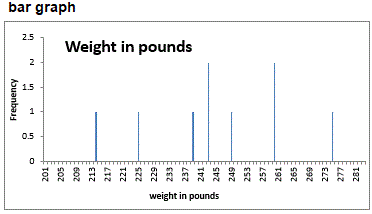
  • BAR GRAPH - a graphic way of displaying each data point and its frequency. It is used for discrete data. On the horizontal axis, the data points are placed on a number line. One the vertical axis frequencies are listed. For each data point, a bar goes from the horizontal axis to the height of the required frequency to display the information.

     
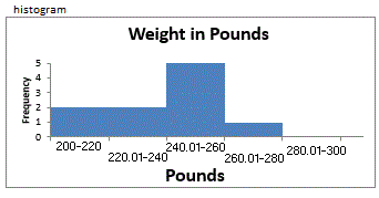
  • HISTOGRAM - a graphic way of displaying intervals of data points and their frequencys. It is used for continuous data. On the horizontal axis, the intervals for the data points are placed on a number line. One the vertical axis frequencies are listed. For each interval, a bar goes from the horizontal axis to the height of the required frequency to display the information. Note: Notice that the histogram has "fat" bars because each number in the interval must be accounted for, whereas a bargraph only displays the data points it needs.

     
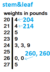
  • STEM-AND-LEAF DIAGRAM - a graphic way of displaying each data point, its frequency, and its position in ordered data. It is used for discrete data. The units digit of each data point is used as a "leaf" and placed on the right off the "tree" of larger digits used as a kind of interval. Each "leaf" in the "stack of leaves" makes the "stack" longer as a frequency bar would.

     
  • CAPITOL SIGMA - - a math symbol meaning "add up the terms."
  • SAMPLE STATICS - numbers, obtained by looking at the sample data in different ways. It is:
            1. used to create a purely numeric picture of the sample,
            2. used to help create the graphic representations of the sample,
            3. used to stand in as a numeric description of the population because none is available,
            4. used in testing if things about the population the sample represents are true.
     
            All of these are sample statistics. Some are used to used to approximate/represent:
     
          1st:   CENTER - "a one number representation" of the entire sample:
    AVERAGE -- any of the following three sample statistics
     
    MEAN -- symbol: , read as "x bar" - arithmetic average. Formula:
     
    MODE -- most frequent score or data point
     
    MEDIAN -- symbol: , read as "x hat" --median, Q2, the 50th percentile, the middle data point when the data is ordered from lowest to highest

          2nd:   SPREAD - "how the data spreads out:
    RANGE - the spread of the data from the highest data point to the lowest data point, xmax - xmin
     
    INNER-QUARTILE RANGE - the spread of the middle 50% of the data, the difference between the 3rd quartile and the 1st quartile, Q3 - Q1, where Q3 is the 75th percentile and Q1 is the 25th percentile. See box-and-whisker with more info.
     
    VARIAVCE - the square of the standard deviation.
     
    STANDARD DEVIATION - the average spread of the data computed in the standard way. The formula is:
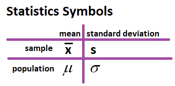
  • STAT SYMBOLS -
  • BOX & WHISKERS PLOT - a drawn to scale representation of how certain sample statistics spread across the sample.

    box-and-whisker with more info

     
  • SYMMETRIC - having a left to right (bilateral) symmetry: the mean or median is in the middle and the tails are the same length and "fattness."
     
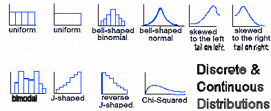
  • Some DISTRIBUTIONS - how the data is spread out, what shape the frequency distribution or histogram has.


Theoretical vs Experimental & Descriptive vs Analytical Statistics

    Thus far only experimental and descriptive statistics (statistics where data is collected, analysed, depicted, and described) has been used. Before analytical statistics (statistics where judgements are made) can be discussed, theoretical statistics (statistics where mathematics and common sense are used to examine a situation) must be discussed.

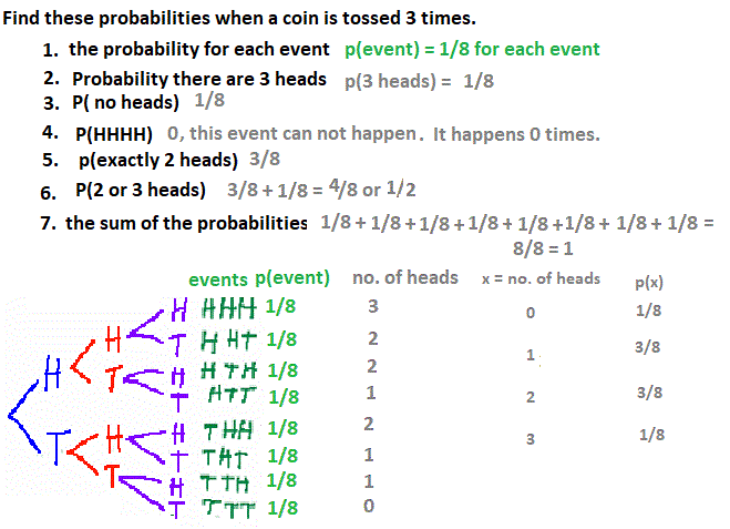
    Your job is to see if common sense and the theoretical statistics agree.

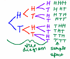
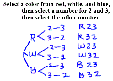
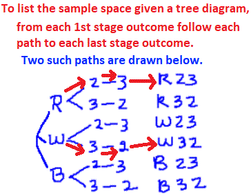
    A tree diageam is a paper and pencil way of figuring out the sample space ( the set of all possible results of an experiment). You can probally guess what each experiment was. Do common sense and the theoretical statistics agree?

Click on the image to go to problems of this sort.

    Why bother with the tree diagram if you can list the sample space in your head? There are reasons:

  1. later you may need justification of your work,
  2. to be sure you list all the possible events, especially in the longer experiments. If you don't need it do not bother, unless,
  3. it gives you credit on a quiz or test.

Vocabulary
  • EXPERIMENTAL & DESCRIPTIVE STATISTICS - statistics where data is collected, analysed, depicted, and described
     
  • THEORETICAL STATISTICS - statistics where mathematics and common sense are used to examine a situation

     
  • TREE DIAGRAM - a paper and pencil way of figuring out the sample space of a multi-step experiment (see above)
          1st: All possible results of the first stage of the experiment are listed vertically on the far left.
          2nd: From each of the first stage events, branches are drawn to the right, to all possible events in the second stage of the experiment.
          This record-keeping continues until all possible outcomes of each stage of the experiment are listed w/branches drawn.
     
  • EVENT - a result, data point, outcome, of an experiment
     
  • SAMPLE SPACE - the set of all possible outcomes/results/events of an experiment

     
  • ANALYTICAL STATISTICS - statistics where judgements are made


Probability

    Before going on, review new vocabulary and vocabulary already discussed.

· experiment -- an action that is performed, like measure a fish
· event -- a result of an experiment
· outcome -- same as event
· sample space -- the set of all possible outcomes or events

    Here's the new stuff.

· probability of an event -- P(event), or p(event)
    ex. p(A), the probability of event A
    ex. p(head), the probability of obtaining a head
    ex. p(x=3), the probability the variable is 3 or
        the probability of the number 3 occuring,
        or the probability of obtaining a 3.
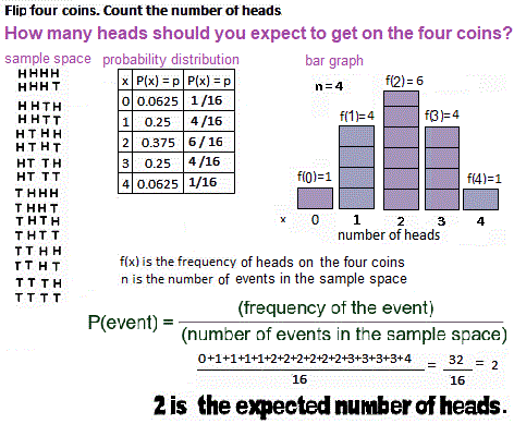
· probability of an event, P(event) = (frequency)/(number) = f/n,
 
(frequency of the event)
P(event) =
 
(number of events in the sample space)

    Here's the answers to some problems. Here are blank problems.

 
Facts
      The lowest possible probability an event might have is 0. If P(event)=0, the event can not happen.
 
      The highest possible probability an event might have is 1. If P(event)=1, the event DOES happen.
 
      Probabilities range between 0 and 1, inclusive.
            0 < P(event) < 1.
 
      The sum of all the probabilities for an experiment is 1. For example:
    ex. Experiment: flip a fair coin.
            P(head) + P(tail) = 1
    ex. Experiment: pick a day of the week.
            p(Sunday) + p(Monday) + ... + p(Saturday) = 7/7 = 1
    ex. Experiment: pick a day of the week
            p(January) = 0
 
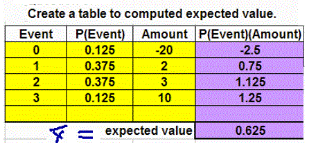
The Expected Value is the Mean.
      One way of describing the results of an experiment is to state the value you expect to get. In any experiment the mean, the arithmetic average, is the expected value.
 
      The expected value is an average. It is the mean.
 
 
      In this case, the expected value is 2, the mean is 2, the mode is 2, and median is 2.
Vocabulary

  • PROBABILITY - a branch of mathemetics that studies populations, samples, experiments, hypothises. It includes experimental, analytical, and theoretical statistics.
     
  • PROBABILITY OF AN EVENT, probability of the data point, or set of numbers, or interval, being the number x, p(x), or being the set of numbers, p(a, b, ..., c), or the inteval, p(athe a number between 0 and 1 that compairs the number of times a specific outcome or event may happen in a situation to the number of possible outcomes in that situation.
          If the probability of the event is 0, the event does not happen.
          If the probability of the event is 1, the event happens.
     
  • EXPECTED VALUE - the mean, the sum of all frequencies divided by the number of possible outcomes
          , the arithmetic average, the sum of the numbers divided by the number of numbers.
         
       
    (the sum of all the data)
      =
     
       
    (number of events in the sample space)


More Vocabulary and Topics that Are Not Included on this Page

    The first 7 definitions are important and understandable without computation.

    The last definitions can not be discussed well, without computation. As promised, these are left out of this page, but references are linked.


Vocabulary

  • INDEPENDENT EVENT - uninfluenced, stand alone, the result of one stage or trial has no effect on another stage or trial.
        ex. Raw sample data - the number of heads when 3 coins are flipped.  The result of each flip, or trial, is not influenced by the other flips.
     
  • DEPENDENT EVENT - having an influence on other stages or trials, the result of one stage of the collection of raw data, has an effect on another stage.
        ex. Raw sample data - the names of a president and vice president of a club with 4 members.
               One officer must be picked at a time or you would not know which officer was which. For instance: There are 4 choices for president, but only 3 choices for vp. The result of the first stage influences the second stage.
     
  • WITH REPLACEMENT - restore the original conditions after each trial. A after a trial or stage, the setting is restored to the original setting before begining the next trial or stage.
        ex. Raw sample data - draw a card from a deck, replace the card in the deck, draw a card from the deck. The 2 draws are independent. The replacement made each draw have the same outcomes.
     
  • WITHOUT REPLACEMENT - do not restore the original conditions after each trial, use the new conditions.
        ex. Raw sample data - draw a card from a deck, draw a 2nd card from the deck.
     
  • ORDER COUNTS - raw data has a 1st, 2nd, 3rd. Ex. officers in a club.
     
  • ORDER DOESN'T COUNT - the order of the raw data does not matter. Ex. a committe (without a chair) is chosen. It doesn't matter how the members are listed.
     
  • FACTORIAL - symbol: n!, the product of a natural number and all the natural numbers less than it, n!=n(n-1)...2·1. See a use on: Number of Ways to Make An Ordered List
    Questions.       Swipe between the stars to see the answer.
    1. 0! is *1, by definition *
    2. 1! is *1 is 1*
    3. 2! is *2x1 is 2*
    4. 3! is *3x2x1 is 6*
    5. 4! is *4x3x2x1 is 24*
    6. 5! is *4x3x2x1 is 120*
    7. 6! is *5x4x3x2x1 is 720*
    8. 7! is *6x5x4x3x2x1 is 5040*
    9. 8! is *8x7x6x5x4x3x2x1 is 40320*
    10. 9! is *9x8x7x6x5x4x3x2x1 is 362880*
    11. 10! is *10x9x8x7x6x5x4x3x2x1 is 3628800*
    The numbers grow quickly. For example 6! is the number of ways 6 people could line up -- order counts.

  •  
  • COUNTING METHODS - Basic Probability & Counting Problems
     
  • PERMUTATIONS - Number of Ways to Make An Ordered List
     
  • COMBINATIONS - Number of Ways to Make A Group


The Binomial Distribution

    Distributions, ways the data in a population is centered and spreads out, have already have been introduced. Now consider one of those distributions in more detail, the Binomial Distribution.


    The binomial is a discrete distribution.

    Raw data is the number, x, of either successes on n identical, independent trials. Again that's:

Binomial distributions have:
  1. n identical trials.
  2. independent trials.
  3. success or failure are the only possible outcomes of each trial.
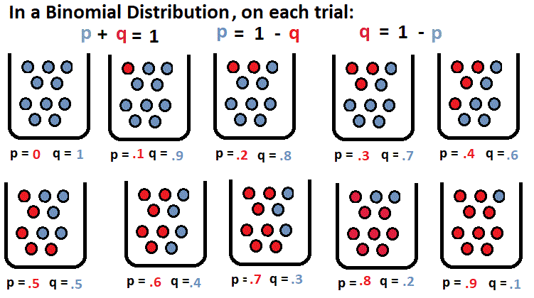
  4. On a trial, p is the probability of success, q is the probability of failure, and since p + q = 1, q = 1- p.

    Probability statements look like p(x=3), meaning the probability of getting exactly 3 heads on n trials.

    The mean and standard deviation of a BINOMIAL DISTRIBUTION are stated below. For an intro to the binomial here's the link. For info on the formulas , click the formulas below. It is all on the same page.

    Think that flipping coins are the only binomial distribution? How about a real-world problem. "Twenty phones have been poorly built. There's a 70% probability that a phone will work when it is switched on. What's the probability that at most half of the machines will run?" Notice that p is now .7 and you now have 20 trials. Harder problem. This kind of problem has not been covered.

    In symbols: Find p(x < 10), p= .7, n=20.


Vocabulary

  • BINOMIAL -- See MIDDLE GROUND - Brief Summary of A Binomial Distribution
     
  • SUCCESS - one of two possible outcomes of a binomial trial. The probability of success is p. Note: p = 1- q
     
  • FAILURE - one of two possible outcomes of a binomial trial. The probability of failure is q. Note: q = 1- p
     
  • DISTRIBUTION - the way the data in a population is centered and spreads out.


Thank Goodness for Probability Density Functions

    Here's a problem for you to do without calculator or computer or spreadsheet:
      You receive a shipment of twenty phones, but have had problems with this supplier before. Last time you got 10 phones, 2 didn't work. What's the probability that at most 4 phones will work?"

    In symbols:
Find p(x < 4) this is
Find p(x < 4) = p(x=1) + p(x=2) + p(x=3) + p(x=4).
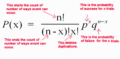
You will need to use the formula below 4 times and then add.
A reasonable q is .2, or 20%. That makes a reasonable p = .8, or 80%.


    I promised light on the computation, so if you want to look at these problems, go to: Binomial Formula Explained.

    Before going back to
"Thank Goodness for Probability Density Functions,"
vocabulary must be examined.

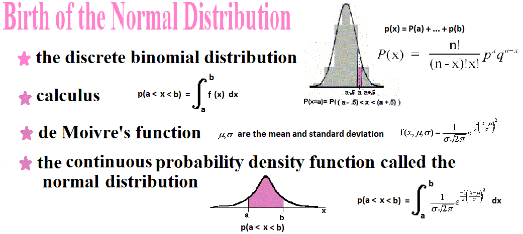
    In 1733, Abraham de Moivre (1667 - 1754) was studying expanding binomials, as in (x + y). See A Binomial Distribution, Explained More Slowly. He was using the discrete binomial distribution and using the above formula multiple times. He realized that with calculus and the right continuous formula for a probability distribution function, f(x), he could use the calculus instead of repeatedly using the binomial formula to easily complete his computation. He wrote such a function. See: History of the Normal Distribution by David M. Lane.    See sheet 9 of: a Calc I Sketchpad


    Johann Carl Friedrich Gauss (177-1855) later worked with the normal distribution. It is named for him. It is also called the bell curve. It is discussed below.


Vocabulary

  • DISTRIBUTION - the way the data is centered and spreads out.
    · the way the numbers in a situation are impacted by the function or rule.
    · Usually the distribution is written algebraically as in f(x) = ...
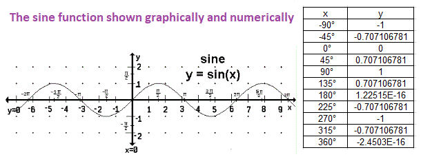
    ex. f(x) = sin(x), the function is the sine of a number

     
  • FUNCTION - a really dependable rule. It is usually written as f(x) where x is the variable, changeable, number
    ex. The area of a rectangle is always the product of its length and width:
              A(l,w) = l(w).
     
  • FREQUENCY - number of occurrences. It reports how many times each specific data point is found in the sample.
     
  • FREQUENCY DISTRIBUTION - a graph showing a table of the frequency of each data point or interval
     
  • RANDOM VARIABLE - a number which is equally likely to be chosen
     
  • INTERVAL - a range of the variable from a number (say a) to a higher number (say b), as in:
    from a to b, a < x < b
    from a to b including a and b, a < x < b
    from a to b including a but not b, a < x < b
    from a to b including b but not a, a < x < b
     
  • CONTINUOUS
     
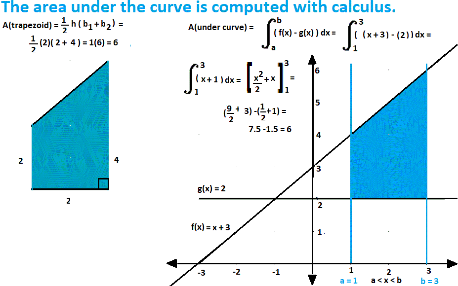
  • AREA UNDER THE CURVE - the sum of all function values, f(x), for each x in the interval. See Statistics Lab 5 - Probabilities for details.

     
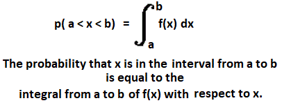
  • PROBABILITY DISTRIBUTION FUNCTION - a continuous function,
    f(x), of probabilities, such that the sum of the probabilities is 1 and:


Normal and Standard Normal Distributions

    Notice in de Moivre's formula for the normal distribution, the notation has gone from:
    f(x) to f(x, , ).

    The variables are x, , and . These are the population random variable, and the constant population mean, and the constant population standard deviation. Everything else in the formula is a constant -- e, and . This is needed because there are really a whole family of normal distributions, each with their own mean and standard deviation, but having the same features.

    In this area of this page, population and sample mean and standard deviation symbols are used. Samples from a normally distributed population will be assumed to be normal also.

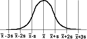
    The mean is always in the center of the symmetric bell-shaped curve. Remember the mean is the measure of center.

    The standard deviation is the measure of spread, the unit on the number line.


For large sets of data that are bell-shaped
(appear normal):
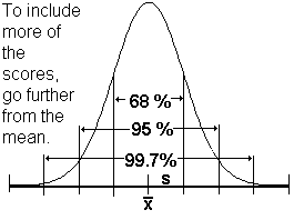
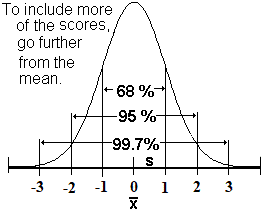
  • 68 % of all scores lie within 1 standard deviation of the mean
    p( - s < x < + s ) = .68
     
  • 95 % of all scores lie within 2 standard deviations of the mean
    p( - 2s < x < + 2s ) = .95
     
  • 99.7% of all scores lie within 3 standard deviations of the mean
    p( - 3s < x < + 3s ) = .997
     

    If your distribution is not normal, bell-shaped, or large, it might be another distribution. There are many.

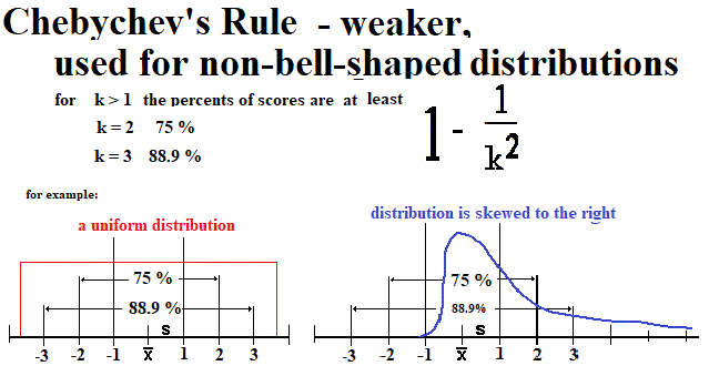
    For percent of scores within k standard deviations of the mean, use Chebychev's Rule.

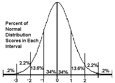
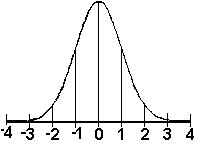
    Even more detail is known about the distribution of normal scores as shown by the image at the left.

    Notice that the mean of this distribution is 0 and the standard deviation is 1.

Questions.       Swipe between the stars to see the answer.
1. What percent of the scores are below the mean? * 50% *
2. What's the probability a score is below the mean? *.5*
3. What's the probability a score is above the mean? *.5*
4. What's the probability a score is equal to the mean?
*0
The probability of getting any one number is 0 because the distribution is defined in terms of an interval. Lines have no thickness, therefore no area, a probability of 0. Intervals have a thickness therefore an area under the curve and a probability.
*
5. The probability p(x>a) = .6, so, what's the probability p( x < a)?
* 1 - .6 = .4, because the sum of these two probabilities must be 1.*
6. What percent of the scores are less than 1 standard deviation above the mean? * 50% + 34% = 84%*


The Standard Normal Distribution

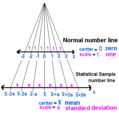
    The number lines at the left are similar. The top one has number labels and the variable is z. The symbol z is used to signify a normal distribution with mean of 0 and standard deviation of 1. It is called the Standard Normal Distribution.

    It is valuable for quick computation and use of statistical tables.

    The bottom number line has the appropriate statistical mean and standard deviation notation. The variable is x.

    Two very useful formulas make it easy to translate x scores into z scores or z into x. Below the calculators do the work for you. Use the percent images above and mental computation or the calculators to answer the questions below the calculators.

Compute x or z
Complete the computation by entering the values and pressing the buttons.
Enter negative two as "-2."
 
 
  -
=
 
 
so,


x = +()()


Questions.          Swipe between the stars for answers.
1. Given the mean is 6, s is 4, and x is 18.
a. Find z *z = 3*
b. Find p(z<3) *p(z<3) = .50 + .34 + .136 + .022 = .998*
c. Find p(x<18) *p(x<18) = .998*
d. Find p(x>18) *p(x>18) = 1 - .998 = .002*
 
2. John needs a 84% or better on the exam to get an A in the course.
The teacher gave the exam before and it has a mean of 75 and a standard deviation of 12.
a. What score does he need on the exam?*x > 87%*

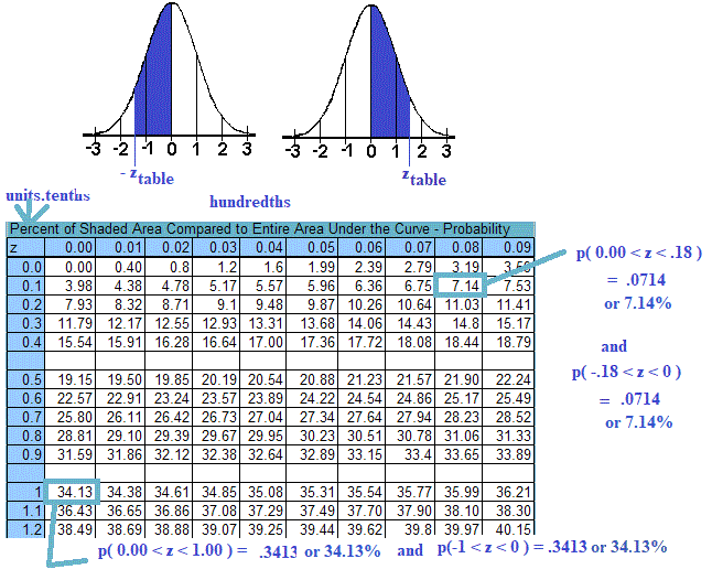
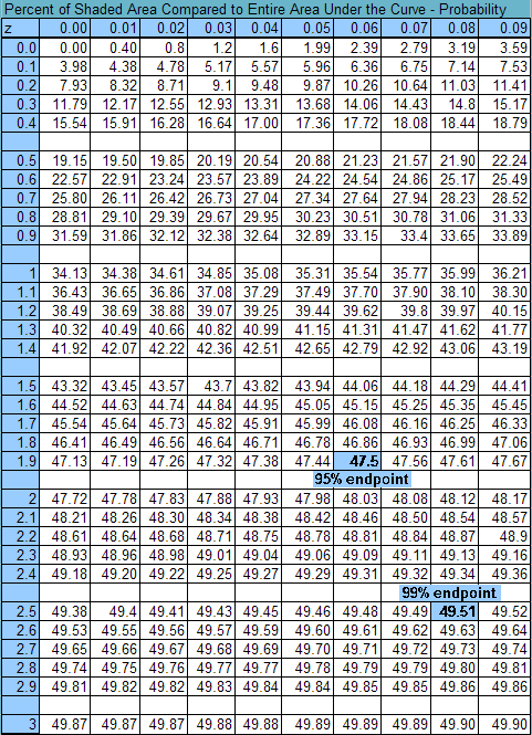
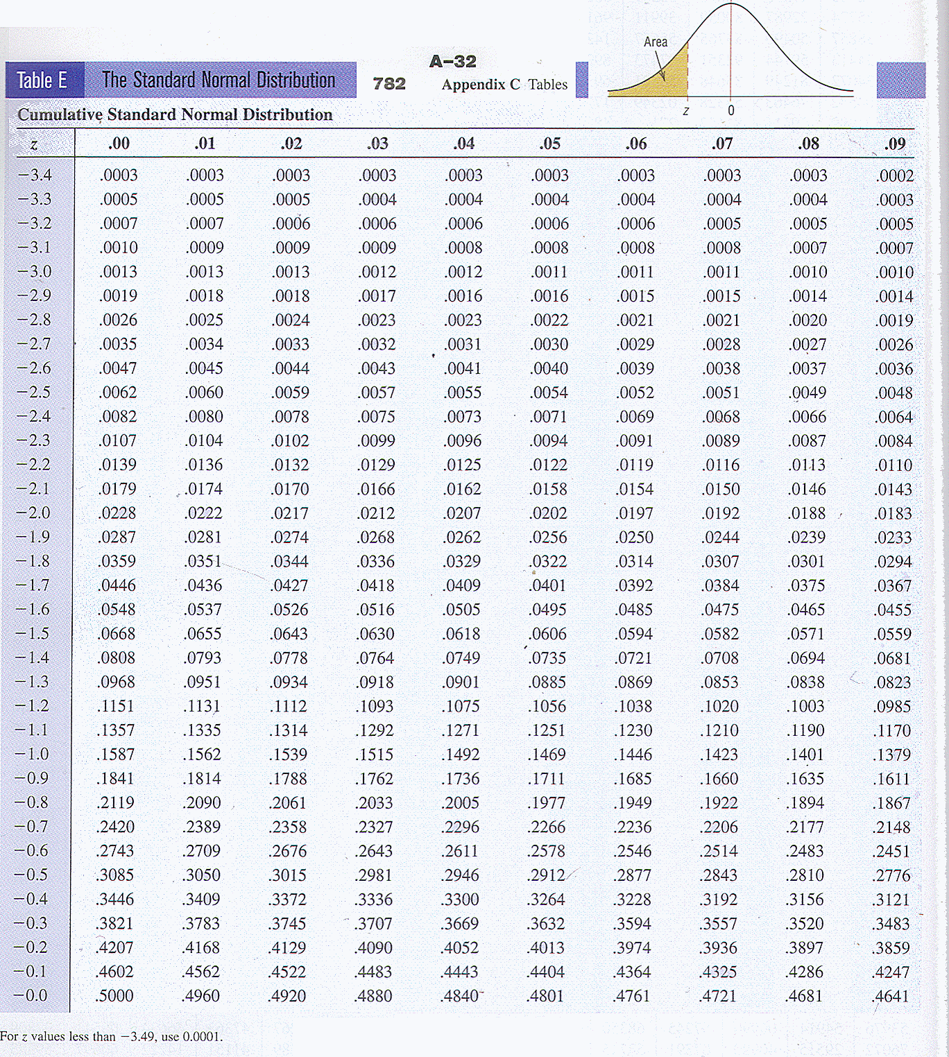
    Now that we've reviewed how the x-score to z-score works and a few of its uses, it is time to examine two tables that have probabilities already computed. Here are the Standard Normal Table of Percents/Probabilities and the Cumulative Standard Normal Distribution. They are on this page to provide a feel for actual probabilities.

    For more info go to Between, Below, Above


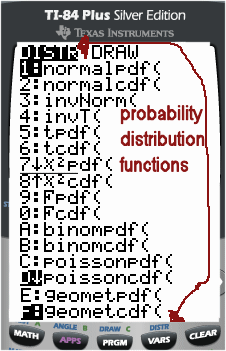
    You may Compute Probabilities Using A Calculator.

    The parameters for a Normal Cumulative Distribution are:
normalcdf(low z, big high z, mean, stdev).


    You may Use the Normal Distribution to Approximate the Binomial.


Vocabulary

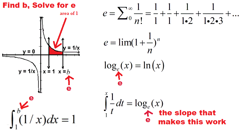
  • e - a constant approximately equal to 2.718281828454590, as defined below.

     
  • z - the variable used to indicate workis with the standard normal distribution having a mean of 0 and a standard deviation of 1.
     
  • PI - - the ratio of the circumference of a circle to its diameter, about 3.14159 or 22/7.
     
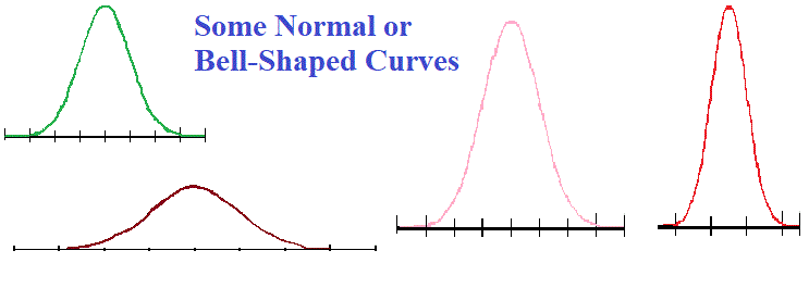
  • NORMAL DISTRIBUTIONS - or Gaussian distribution, a continuous probability distribution (so the area under the curve equals 1), where the mean, mode, median are all the same, so the data gathers about a center making a symmetric bell-shaped curve. Many data points -- heights of people, lengths of fish, errors measurements, standardized test scores have normal distributions.

     
  • STANDARD NORMAL DISTRIBUTION - a normal distribution having a mean of 0 and a standard deviation of 1. It is very useful in computing, and looking up, probabilities, comparing samples and populations, and analysis and hypothesis testing.

     
  • STANDARD NORMAL TABLE OF PERCENTS/PROBABILITIES - uses z-scores and their probabilities.

     
  • CUMULATIVE STANDARD NORMAL DISTRIBUTION - uses z-scores and their probabilities beginning with z=-3 and ending with z= 3 but, lists the sum of the probabilities from z = -3 to the desired z-score.

     
  • BELL-SHAPED CURVE - a normal distribution. It looks like a symmetric bell sitting on a table. The scores are piled in the center and trail off at the upper and lower range of variables.

     
  • WITHIN A SPECIFIC STANDARD DEVIATION OF THE MEAN - a range of scores centered about the mean and, in either direction, not farther on the number line than the specified number of standard deviations.
     
    ex. on the standard normal number line, "within 1 standard deviation of the mean" means, from -1 to 1, - 1 < z < 1, and includes about 68% of the scores
     
    ex. on the normal number line, "within 3 standard deviation of the mean" means, from -3 to 3, - 3 < x < 3, and includes about 99.7% of the scores.


  • CHEBYCHEV'S RULES -- for any distribution, the percent of scores within k standard deviations of the mean, k > 0, is 1/k2


Confidence Interval

    Before making a claim, most people like to be sure, or pretty sure, the statement is true. The statement might be about the mean of the population being sampled, or a belief one treatment has a higher mean than another, or that the means of 3 or more populations are the same.

    One might be 90% confident or sure about the statement, 95% condifent, etc. The larger the sample, the more sure or confident one would be about one's statement.

    Making a statement and stating how confident one is about the statement go hand-in-hand in statistics.


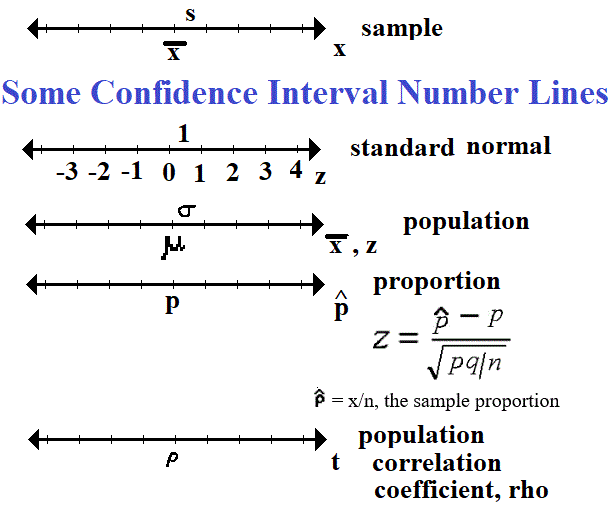
    At the left is a number line on which an interval has been drawn.

    Since it is unlabeled it might be
25 < x < 45, or 25 < < 45, or
25 < < 45, or something else. Which one is used depends on what is studied or sampled or tested.

    Below that are a bunch of number lines which are labeled for use as what is called a confidence interval. You should be familiar with the top three number lines.

More below.


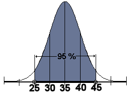
    At the left a curve that looks like a normal probability density function or a frequency distribution has been added.

    It's mean, mode, and median are all the same. It looks like 95% of the scores lie within what looks like 2 standard deviations. It is bell-shaped and symmetric.

    Call it a normal distribution of sample means, like number line 3 above, used to estimate the population mean. Note it is labeled as having 95% of the scores within the interval.

    From 25 to 45 is the confidence interval for this normal distribution having a 95 % level of confidence. A confidence interval is the range of score in which you believe the population parameter is found.

    If the confidence interval accounts for 95 % of the scores, what percent of the scores under the density function are not in the interval, but out in the tails?
*5 %, 1 - .95 = .05, or 5 %*

    Old Symbols:
  • population mean, (mu),
  • population standard deviation, (sigma),
  • z, the standard normal variable
        (mean of 0, standard deviation of 1),
        used in a bunch of stuff including probability tables.
    New Symbols:
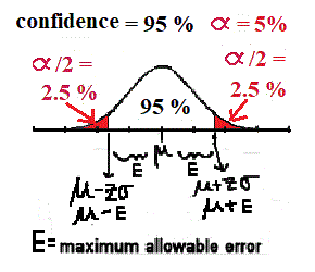
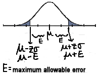
  • E, the error, the maximum distance from the mean that still places a score within the confidence interval
  • (alpha) - the area under the density function which is not in the confidence interval.
        Sometimes alpha is in the two tails and other times alpha is only in one tail.
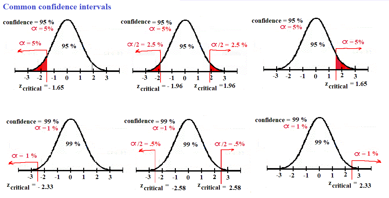
    Below are often-used confidence intervals marked with:
  • a z-score number line,
  • the degree of confidence,
  • alpha, "(1- degree of confidence),"
        the probability a score does not fall into the confidence interval
  • the critical z-scores, the endpoints of the confidence interval with the desired level of confidence.

Vocabulary

  • CONFIDENCE INTERVAL - range of expected values, a range of score in which the population parameter is believed to be.
     
  • alpha, - "(1- degree of confidence)," the probability a score does not fall into the confidence interval
     
  • LEVEL OF CONFIDENCE - in the picture below P( - E < < + E) -- a probability, usually expressed as a percent, that states how sure one is about the decision made by the test.
        ex. Test with a 90% level of confidence that > 60, with -- probability a score is in the confidence interval containing the mean.

     
  • E, error -- the maximum distance from the mean that still places a score within the confidence interval . (See above image.)


Hypothesis Testing

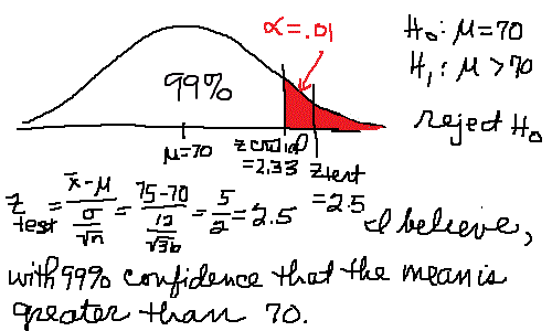
    Your mother, the math teacher, says your fish are getting too big.

    She says, "They were on average 70 mm long when you got them. You've been feeding them. They've been growing. They are getting too big for the tank."

    You say, "No. They are fine. They're still on average 70 mm long."

    "Ok. We need more information," said the mother. "One of my former students sold us the fish. He was really into statistics and wrote some population parameters on the receipt which I kept."

    "Your fish tank population mean length was 70 mm, which you already knew. The population standard deviation was 12 mm and you got about 80 fish."

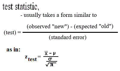
    "Take 36 fish for a sample. Measure them as accurately as you can. We'll assume the population is normal and you can run a Hypothesis Test so we can make a judgement based on statistics. Here's a formula for your test statistic. When you finish, we'll see about the fish."

    You have no idea what she's talking about!


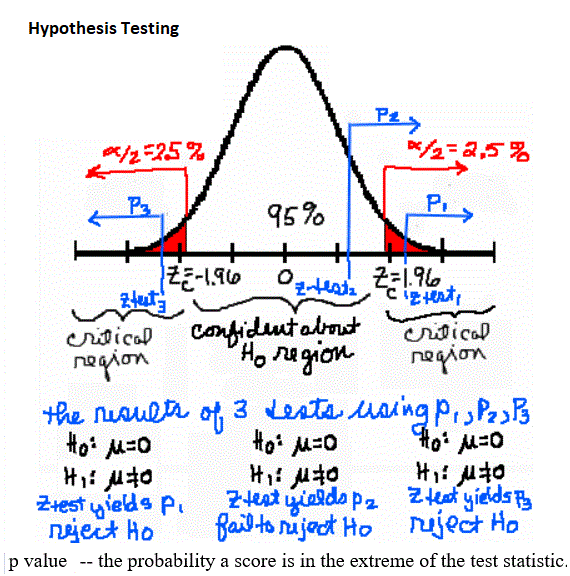
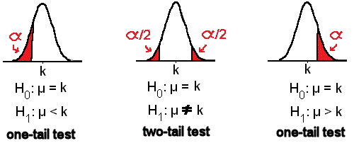
    Before examining how to complete a hypothesis test, examing closely the picture below. Click on the picture to enlarge it.

    Old Symbols:
  • population mean, (mu),
  • population standard deviation, (sigma),
  • z, the standard normal variable
  • (alpha) - the area under the density function which is not in the confidence interval.
        Sometimes alpha is in the two tails and other times alpha is only in one tail.
    New Symbols:
  • k-- constant, like 70, ex. = 70
  • hypothesis (no symbol) -- a theory or statement which may or may not be true
  • H0 -- read as "H 0" -- the null (original or beginning) hypothesis
  • H1 -- read as "H 1" -- the alternate (new) hypothesis

    A hypothesis test is a procedure by which a hypothesis (or statement) which one believes to be true is tested statistically against another hypothesis already in use.

    Before clarification of this, some questions.

Questions.       Swipe between the stars to see the answer.
 
1. In the fish tank story, write the tank owner's hypothesis in symbols.
* H0 = 70*
2. In the fish tank story, write the mother's hypothesis in symbols.
* H1 > 70*
3. Will the test be a one-tail test or a two-tail test? *1*
4. Use the image Common confidence intervals which you have seen before.
Find and state the number that is labeled zcritical at the 95% confidence level.*zcritical = 1.65*
5. Use the image Common confidence intervals which you have seen before.
Find and state the number that is labeled zcritical at the 99% confidence level.*zcritical = 2.58*
6. Where did these zcritical numbers come from before they were put on the image?
*the table of probabilities given the z-score* See it.

    At the left additional z-critical values are listed.

    They were also retrieved from the probability table.


    Here's where we are so far:
  • A hypothesis test is
        a procedure by which a hypothesis (or statement) which one believes to be true is tested statistically against another hypothesis already in use.
  • The population is normal.
  • = 70
  • = 12
  • N = 80, approximately
  • H0 = 70
  • H1 > 70
  • - as yet undetermined.
        We will use = .01, or 1 %
        Level of confidence is 99%.
        zcritical = 2.33
  • n = 36
  • ztest =????
        Must compute the ztest

    The calculator below has been provided to do the computation for you. Please use it to compute ztest.


   Compute z-test.   
Complete the computation by entering the values and pressing the buttons.
Enter negative two as "-2."
 

( - )

=
 

(/ )

 
so,

    As soon as you realize ztest is not in the confidence interval but out in the tail, the alpha region, larger than the zcritical, you know it's likely your mother was right, with 99% confidence.

    But you could be right.

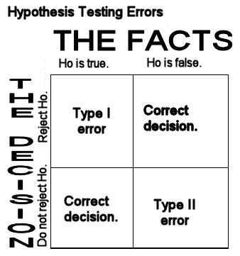
    Thereare two kinds of statistical errors with a hypothesis test, Type I and type II.

    Type II error means "When the null hypothesis is false, you do not reject it."

    Type I error means "When the null hypothesis is true, you reject the null hypothesis." This would be the case if the mean fish length were 70 mm as you believe, but the test results indicate that your mother's hypothesis that the mean is greater than 70 mm was the one indicated.

    You did not but could have made a math mistake in choosing a two-tail test rather than the one-tail test you chose for your test.


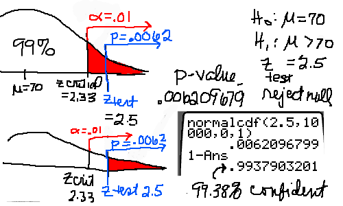
    Notice on the left a new symbol has been introduced in blue.

    It is the "p value," the probability a score is in the extreme of the test statistic.
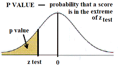
    You can get the p value using either your calculator or the Cumulative Standard Normal Distribution.

    There are many different hypothesis tests because there are many situations in which new information or verification is desired. We have been looking at a Z-Test for Normal Density Functions. For additional information on how to run a test see Hypothesis Testing.

    Before continuing, a summary of a test is needed. You need:
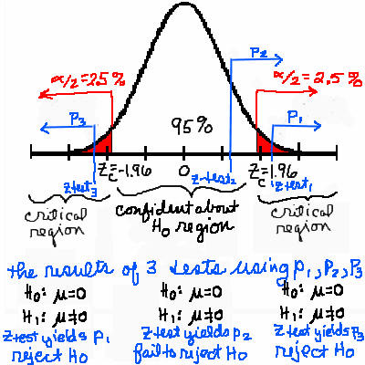
  • a reason to run the test.
      Perhaps, you believe a mean is incorrect, you think that two means or two probabilities (as in "70% of males," vs "42% of females") are different, ...
  • specific information about the situation.
  • to decide if a one-tailed or two-tailed test is needed.
  • to compute a test statistic.
  • to compute either zcritical or a p value.
  • to make a decision about your hypothesis.

    Now, examine other hypothesis tests the web page, or, HYPOTHESIS TESTS pdf file or video about the HYPOTHESIS TESTS pdf file, yes, a video about a pdf file, filed with other videos.

    You have completed "A Year of Statistics in an Hour or Two." Stay safe. --A2


Vocabulary

  • k-- constant, like 70, ex. = 70
     
  • HYPOTHESIS (no symbol) -- a theory or statement which may or may not be true
  • HYPOTHESIS TEST - a procedure by which a hypothesis (or statement) which one believes to be true is tested statistically against another hypothesis already in use.
     
  • NULL HYPOTHESIS - H0 -- read as "H 0" -- the null (original or beginning) hypothesis
     
  • ALTERNATE HYPOTHESIS - H1 -- read as "H 1" -- the alternate (new) hypothesis
     
  • ONE-TAIL TEST - used when the alternate hypothesis, H1, is k, where k is the null hypothesis mean.
     
  • TWO-TAIL TEST - used when the alternate hypothesis, H1, is > k or < k, where k is the null hypothesis mean.
     
  • Z-CRITICAL - zcritical -- the boundary value(s) which end the confidence interval.
     
  • Z-TEST -- the evidence used to accept or reject the null hypothesis, usually computed from sample data.
     
  • TYPE I ERROR - "When the null hypothesis is true, you reject the null hypothesis."
     
  • TYPE II ERROR - -- "When the null hypothesis is false, you do not reject it."

     
  • P VALUE - the probability a score is in the extreme of the test statistic.

     
Just vocabulary.

Vocabulary


Class Table [MC,i. Home] [Table] [Words] Classes [this semester's schedule w/links] [Good Stuff -- free & valuable resources]
© 2018, 2021, 2022, A. (a^2) Azzolino
www.mathnstuff.com/math/spoken/here/2class/90/fish.htm