MIDDLE GROUND - Binomial Formula Explained

 

Use the Normal to Compute the Binomial.         Using the normal to compute the binomial is an important mathematical idea but now an old computational technique. For the most part, calculators functions have replaced statistical tables as sources for values of probability distributions.         It is valuable to know that for large values of n, the discrete binomial distribution approaches the continuous normal distribution.         When n(p) >5 and n(q) >5, the normal distribution may be used to approximate the binomial. This technique is useful when: binomial tables are not available for the given n, the numbers for n is large, or computation is required for more than 1 value of x, as in p(x>2), since repeated use of the formula or even the tables might be a pain.       The normal distribution does not match the binomial distribution, but, for larger values of n the shape matches closer and closer.         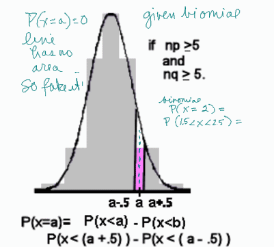In each distribution, the probability is the area under the curve. For the binomial distribution (which is discrete), each value of x has a thickness on the x axis. For the normal distribution (which is continuous), each value of x has one one point on the x-axis where a vertical line crosses the axis.         Since a line does not have an area (the vertical line x=2 to compute p(x=2), for example), one must use an interval (the interval 1.5 < x < 2.5 to compute p(1.5 < x < 2.5), for example) to compute the probability.         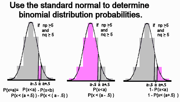Because of the above, to use this technique, one must rewrite the binomial probability expression to match an expression which can be evaluated by a normal probability expression.         This technqiue requires taking the statement of equality (one which inlcudes =) and rewriting it as a statement of inequality (one which includes >, <, >, or <, or multiple statements of inequality. The figures below depict this technique.

 

Compute Using A Calculator         The Distribution menu, [DISTR], lists probability distribution functions. It is found above the Varibles menu, [2nd] [VARS].         Funtion A, listed as [A:binomcdf(], is the cumulative BINOMIAL distribution. It is similar to the NORMAL cumulative distribution funtion, [2:normalcdf(]. It adds "from the left."           Each function requires parameters, stated in specific order and manner, for the function to work.         If p is the probability of success and x is the number of successes on n trials, the cumulative binomial distribution is computed using binomcdf(n,p,x) where , is the comma key, [,].         To compute p(x<1) where n is 4 and p is .4, use         binomcdf(4,.4,1).         This value is .4752 and is shown below on a calculator home screen and in a written-upon binomial distribution table.

 

 

© 2010, Agnes Azzolino www.mathnstuff.com/math/spoken/here/2class/90/binom6.htm